LUMI Performance Workshop - Stockholm, Sweden (May 2026)¶

ssh USERNAME@lumi.csc.fi

To simplify the login to LUMI, you can add the following to your .ssh/config file.

# LUMI
Host lumi
User <USERNAME>
   Hostname lumi.csc.fi
   IdentityFile <HOME_DIRECTORY>/.ssh/id_rsa 
   ServerAliveInterval 600
   ServerAliveCountMax 30

The ServerAlive* lines in the config file may be added to avoid timeouts when idle.

Now you can shorten your login command to the following.

ssh lumi

During the course only:¶

If you are able to log in with the ssh command, you should be able to use the secure copy command to transfer files. For example, you can copy the presentation slides from lumi to view them. project_465002770

scp lumi:/project/project_465002770/Slides/AMD/<file_name> <local_filename>

You can also copy all the slides with the . From your local system:

mkdir slides
scp -r lumi:/project/project_465002770/Slides/AMD/* slides

If you don't have the additions to the config file, you would need a longer command:

mkdir slides
scp -r -i <HOME_DIRECTORY>/.ssh/<public ssh key file> <username>@lumi.csc.fi:/project/project_465002770/slides/AMD/ slides

or for a single file

scp -i <HOME_DIRECTORY>/.ssh/<public ssh key file> <username>@lumi.csc.fi:/project/project_465002770/slides/AMD/<file_name> <local_filename>

After the course:¶

All materials are also available via the course pages on the training website. Slides can be found at their respective talks and exercises can be installed from a downloadable tar file.

HIP Exercises¶

We assume that you have already allocated resources with salloc

While the course project is active, you can get the examples with

cp -r /project/project_465002770/Exercises/AMD/HPCTrainingExamples/ .

After the course, follow the instructions on the course page on the training website.

salloc -N 1 -p standard-g --gpus=1 -t 10:00 -A project_46YXXXXXX

module load craype-accel-amd-gfx90a
module load PrgEnv-amd
module load rocm

The examples are also available on github:

git clone https://github.com/amd/HPCTrainingExamples

Alternatively, you can copy them from Exercises/AMD/HPCTrainingExamples after uncompressing the downloadable tar-archive of the exercises.

Basic examples¶

cd HPCTrainingExamples/HIP/vectorAdd

Examine files here – README, Makefile and vectoradd_hip.cpp Notice that Makefile requires HIP_PATH to be set. Check with module show rocm or echo $HIP_PATH Also, the Makefile builds and runs the code. We’ll do the steps separately. Check also the HIPFLAGS in the Makefile.

export HCC_AMDGPU_TARGET=gfx90a
make
srun -n 1 ./vectoradd

We can use SLURM submission script, let's call it hip_batch.sh:

#!/bin/bash
#SBATCH -p standard-g
#SBATCH -N 1
#SBATCH --gpus=1
#SBATCH -t 10:00
#SBATCH -A project_46YXXXXXX

module load craype-accel-amd-gfx90a
module load rocm
cd $PWD/HPCTrainingExamples/HIP/vectorAdd 

export HCC_AMDGPU_TARGET=gfx90a
make vectoradd
srun -n 1 --gpus 1 ./vectoradd

Submit the script

sbatch hip_batch.sh

Check for output in slurm-<job-id>.out or error in slurm-<job-id>.err

Compile and run with Cray compiler

CC -x hip vectoradd.hip -o vectoradd
srun -n 1 --gpus 1 ./vectoradd

Now let’s try the cuda-stream example from https://github.com/ROCm-Developer-Tools/HIP-Examples. This example is from the original McCalpin code as ported to CUDA by Nvidia. This version has been ported to use HIP. See add4 for another similar stream example.

git clone https://github.com/ROCm/HIP-Examples
export HCC_AMDGPU_TARGET=gfx90a
cd HIP-Examples/cuda-stream
make
srun -n 1 ./stream

Note that it builds with the hipcc compiler. You should get a report of the Copy, Scale, Add, and Triad cases. The variable export HCC_AMDGPU_TARGET=gfx90a is not needed in case one sets the target GPU for MI250x as part of the compiler flags as --offload-arch=gfx90a.

Now check the other examples in HPCTrainingExamples/HIP like jacobi etc.

Hipify¶

We’ll use the same HPCTrainingExamples that were downloaded for the first exercise.

Get a node allocation.

salloc -N 1 --ntasks=1 --gpus=1 -p standard-g -A project_46YXXXXXX –-t 00:10:00

A batch version of the example is also shown.

Hipify Examples¶

Exercise 1: Manual code conversion from CUDA to HIP (10 min)¶

Choose one or more of the CUDA samples in HPCTrainingExamples/HIPIFY/mini-nbody/cuda directory. Manually convert it to HIP. Tip: for example, the cudaMalloc will be called hipMalloc. Some code suggestions include nbody-block.cu, nbody-orig.cu, nbody-soa.cu

You’ll want to compile on the node you’ve been allocated so that hipcc will choose the correct GPU architecture.

Exercise 2: Code conversion from CUDA to HIP using HIPify tools (10 min)¶

Use the hipify-perl script to “hipify” the CUDA samples you used to manually convert to HIP in Exercise 1. hipify-perl is in $ROCM_PATH/bin directory and should be in your path.

First test the conversion to see what will be converted

hipify-perl -no-output -print-stats nbody-orig.cu

You'll see the statistics of HIP APIs that will be generated.

[HIPIFY] info: file 'nbody-orig.cu' statistics:
  CONVERTED refs count: 7
  TOTAL lines of code: 82
  WARNINGS: 0
[HIPIFY] info: CONVERTED refs by names:
  cudaFree => hipFree: 1
  cudaMalloc => hipMalloc: 1
  cudaMemcpy => hipMemcpy: 2
  cudaMemcpyDeviceToHost => hipMemcpyDeviceToHost: 1
  cudaMemcpyHostToDevice => hipMemcpyHostToDevice: 1

hipify-perl is in $ROCM_PATH/bin directory and should be in your path.

Now let's actually do the conversion.

hipify-perl nbody-orig.cu > nbody-orig.cpp

Compile the HIP programs.

hipcc -DSHMOO -I ../ nbody-orig.cpp -o nbody-orig

The #define SHMOO fixes some timer printouts. Add --offload-arch=<gpu_type> if not set by the environment to specify the GPU type and avoid the autodetection issues when running on a single GPU on a node.

Fix any compiler issues, for example, if there was something that didn’t hipify correctly.
Be on the lookout for hard-coded Nvidia specific things like warp sizes and inlined PTX code.

Run the program

srun ./nbody-orig

A batch version of Exercise 2 is:

#!/bin/bash
#SBATCH -N 1
#SBATCH --ntasks=1
#SBATCH --gpus=1
#SBATCH -p standard-g
#SBATCH -A project_46YXXXXXX
#SBATCH -t 00:10:00

module load craype-accel-amd-gfx90a
module load rocm

export HCC_AMDGPU_TARGET=gfx90a

cd HPCTrainingExamples/mini-nbody/cuda
hipify-perl -print-stats nbody-orig.cu > nbody-orig.cpp
hipcc -DSHMOO -I ../ nbody-orig.cpp -o nbody-orig
srun ./nbody-orig
cd ../../..

Notes:

Hipify tools do not check correctness
hipconvertinplace-perl is a convenience script that does hipify-perl -inplace -print-stats command

Rocprof¶

Setup environment

salloc -N 1 --gpus=8 -p standard-g --exclusive -A project_46YXXXXXX -t 20:00

module load PrgEnv-cray
module load craype-accel-amd-gfx90a
module load rocm

Obtain examples repo and navigate to the HIPIFY exercises

cd HPCTrainingExamples/HIPIFY/mini-nbody/hip/

Compile and run one case. We are on the front-end node, so we need to point he tools to use the correct GPU:

export HCC_AMDGPU_TARGET=gfx90a

have two ways to compile for the GPU that we want to run on. We can now complete the build with:

make nbody-orig

Now Run rocprof on nbody-orig to obtain hotspots list

srun rocprof --stats nbody-orig 65536

Check Results

cat results.csv

Check the statistics result file, one line per kernel, sorted in descending order of durations

cat results.stats.csv

Using --basenames on will show only kernel names without their parameters.

srun rocprof --stats --basenames on nbody-orig 65536

Check the statistics result file, one line per kernel, sorted in descending order of durations

cat results.stats.csv

Trace HIP calls with --hip-trace

srun rocprof --stats --hip-trace nbody-orig 65536

Check the new file results.hip_stats.csv

cat results.hip_stats.csv

Profile also the HSA API with the --hsa-trace

srun rocprof --stats --hip-trace --hsa-trace nbody-orig 65536

Check the new file results.hsa_stats.csv

cat results.hsa_stats.csv

On your laptop, download results.json

scp -i <HOME_DIRECTORY>/.ssh/<public ssh key file> <username>@lumi.csc.fi:<path_to_file>/results.json results.json

Open a browser and go to https://ui.perfetto.dev/. Click on Open trace file in the top left corner. Navigate to the results.json you just downloaded. Use the keystrokes W,A,S,D to zoom in and move right and left in the GUI

Navigation
w/s Zoom in/out
a/d Pan left/right

Read about hardware counters available for the GPU on this system (look for gfx90a section)

less $ROCM_PATH/lib/rocprofiler/gfx_metrics.xml

Create a rocprof_counters.txt file with the counters you would like to collect

vi rocprof_counters.txt

Content for rocprof_counters.txt:

pmc : Wavefronts VALUInsts
pmc : SALUInsts SFetchInsts GDSInsts
pmc : MemUnitBusy ALUStalledByLDS

Execute with the counters we just added:

srun rocprof --timestamp on -i rocprof_counters.txt  nbody-orig 65536

You'll notice that rocprof runs 3 passes, one for each set of counters we have in that file.

Contents of rocprof_counters.csv

cat rocprof_counters.csv

Exploring Rocprofiler-v3¶

ROCm 6.3.4 - LUMI default is in the transition Rocprof (v1) to Rocprofv3 so we recommend users adopt the new tool as it is becoming default in ROCm 6.4. If you wich trying more recnet version, e.g., ROCm 6.4.2 you can execute:

module use /appl/local/containers/test-modules
module load rocm/6.4.4

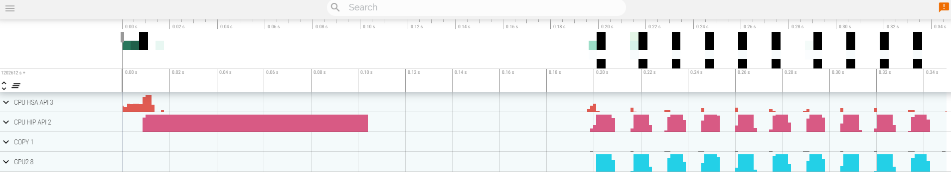
We can now repeat the experiment we did before and obtain a HIP trace with the kernels and copy information:

srun rocprofv3 --hip-trace --kernel-trace --memory-copy-trace --output-format=pftrace -- ./nbody-orig 65536

Notice the difference in the options in comparison to rocprof V1. One can be more selective on what to collect. You would also notice that the profiler is faster and has less overhead. It also has the choice of using pftrace format that are more compatible with latest versions of the Perfetto UI https://ui.perfetto.dev/. The trace will look similar to what seen before with a slightly different convention for the namming of the different sections:

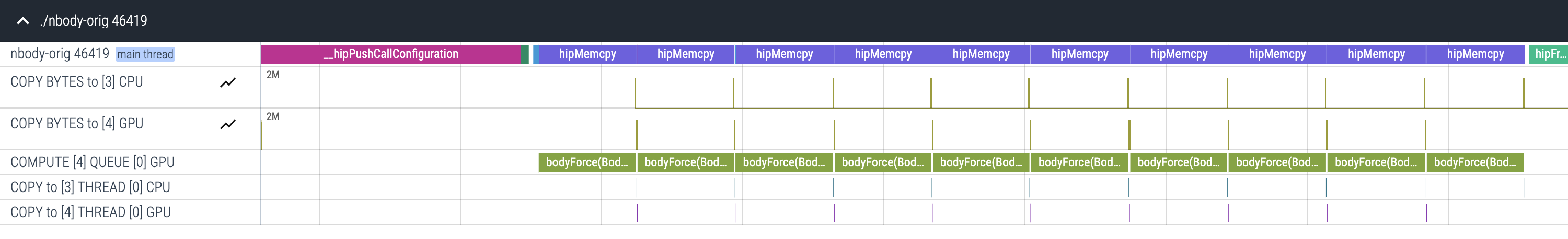
For convinience, the result files are located in a subfolder named after the node where it was run, e.g., nid<node ID>/<process ID>_results.pftrace. The tool should print the full path when it completes so you can just copy that to your workstation.

Rocprof-sys¶

Load suitable ROCm version

Rocprof-sys is packaged with ROCm distribution. However, the default ROCm instalation on LUMI decided to not include that - so we use a different ROCm installation to provide the extra tools:
```
module load craype-accel-amd-gfx90a
module load PrgEnv-amd
module load cray-python

module use /appl/local/containers/test-modules
module load rocm/6.4.4
```

Allocate resources with salloc

salloc -N 1 --ntasks=1 --partition=standard-g --gpus=1 -A project_46YXXXXXX  --time=00:15:00

Check the various options and their values and also a second command for description

srun -n 1 --gpus 1 rocprof-sys-avail --categories rocprofsys

srun -n 1 --gpus 1 rocprof-sys-avail --categories rocprofsys --brief --description

Create an Rocprof-sys configuration file with description per option
```
srun -n 1 rocprof-sys-avail -G rocprofsys.cfg --all
```

Declare to use this configuration file:

export ROCPROFSYS_CONFIG_FILE=$(realpath rocprofsys.cfg)

Get the training examples:
```
cp -r /project/project_465002770/Exercises/AMD/HPCTrainingExamples/ .
```
or according to the instructions on the course page on training website after the course.

Compile and execute saxpy

cd HPCTrainingExamples/HIP/saxpy

hipcc --offload-arch=gfx90a -O3 -o saxpy saxpy.hip

time srun -n 1 ./saxpy

Check the duration

Compile and execute Jacobi

cd HPCTrainingExamples/HIP/jacobi

Now build the code (needs a couple of changes to accomodate the system MPI implementation)

sed -i 's/USE_CRAYPE=.*/USE_CRAYPE=yes/g' Makefile

sed -i 's/IS_MPICH=.*/IS_MPICH=yes/g' Makefile

make -f Makefile

time srun -n 1 --gpus 1 Jacobi_hip -g 1 1

Check the duration

Dynamic instrumentation (the commands take a significant ammount of time)¶

Execute dynamic instrumentation on the saxpy example:
```
cd HPCTrainingExamples/HIP/saxpy
```
```
time srun -n 1 -c 7 --gpus 1 rocprof-sys-instrument -- ./saxpy
```
Check the duration - you'd seeing the instrumentation overhead.
Execute dynamic instrumentation on the Jacobi example:
```
cd HPCTrainingExamples/HIP/jacobi
```
```
time srun -n 1 -c 7 --gpus 1 rocprof-sys-instrument -- ./Jacobi_hip -g 1 1
```
Check the duration - it will take a while. that is the point of this exercise: instrumenting is time consuming.
About Jacobi example, as the dynamic instrumentation would take long time, check what the binary calls and gets instrumented:
```
nm --demangle Jacobi_hip | egrep -i ' (t|u) '
```

Available functions to instrument:

srun -n 1 -c 7 --gpus 1 rocprof-sys-instrument -v 1 --simulate --print-available functions -- ./Jacobi_hip -g 1 1

the simulate option means that it will not execute the binary

Binary rewriting (to be used with MPI codes and decreases overhead)¶

Binary rewriting:

srun -n 1 --gpus 1 rocprof-sys-instrument -v -1 --print-instrumented functions -o jacobi.inst --function-include Jacobi -- ./Jacobi_hip

We created a new instrumented binary called jacobi.inst

Activate text profile logic in your configuration file:
```
ROCPROFSYS_PROFILE = true
```

Executing the new instrumented binary:

time srun -n 1 --gpus 1 rocprof-sys-run -- ./jacobi.inst -g 1 1

and check the duration

See the duration of the instrumented calls as well as GPU runtime activity:
```
cat rocprofsys-jacobi.inst-output/TIMESTAMP/wall_clock-0.txt
```

Visualization¶

Copy the perfetto-trace.proto to your laptop, open the web page https://ui.perfetto.dev/. Click to open the trace and select the file.

Hardware counters¶

See a list of all the counters:

srun -n 1 --gpus 1 rocprof-sys-avail --all

Declare in your configuration file: ROCPROFSYS_ROCM_EVENTS = _
Execute: l and copy the perfetto file and visualize

Sampling¶

Activate in your configuration file ROCPROFSYS_USE_SAMPLING = true and ROCPROFSYS_SAMPLING_FREQ = 100, execute and visualize. You should be able to see call-stack information as part of your trace.

You can execute the plain binary as sampling does not require prior instrumentation:

srun -n 1 --gpus 1 rocprof-sys-run -- ./Jacobi_hip  -g 1 1

Kernel timings¶

Open the file rocprofsys-<binary>-output/timestamp/wall_clock-0.txt (replace binary and timestamp with your information)
In order to see the kernels gathered in your configuration file, make sure that ROCPROFSYS_PROFILE = true and ROCPROFSYS_FLAT_PROFILE = true, execute the code and open again the file rocprofsys-<binary>-output/timestamp/wall_clock-0.txt

Rocprof-compute¶

Load and prepare Rocprof-compute:

Rocprof-compute uses a separate instalation as it is not part of ROCm default instalation. Let's load it in our environment.
```
module load craype-accel-amd-gfx90a
module load PrgEnv-amd
module load cray-python

module use /appl/local/containers/test-modules
module load rocm/6.4.4
```
There are some Python dependencies needed. The tool is not assuming a particular Python version as that should be compatible with workload (it it uses Python). for simplicity we use an existing Python version provided by the cray-python module. The extra packages can be loaded into your environment with:
```
python3 -m venv venv
source venv/bin/activate
pip install -r $ROCM_PATH/libexec/rocprofiler-compute/requirements.txt
```
Reserve a GPU, compile the exercise and execute rocprof-compute, observe how many times the code is executed. Note that we use rocprofv2 to collect the data. We could use rocprofv3 but that requires all GPUs in the node visible - this is a limitation that will be lifted in more recent version.
```
salloc -N 1 --ntasks=1 --partition=small-g --gpus=1 -A project_465002770 --time=00:30:00
cp -r /project/project_465002770/Exercises/AMD/HPCTrainingExamples/ .
source venv/bin/activate
cd HPCTrainingExamples/HIP/dgemm/
mkdir build
cd build
cmake ..
make
cd bin
ROCPROF=rocprofv2 srun -n 1 --gpus 1 rocprof-compute profile -n dgemm -- ./dgemm -m 8192 -n 8192 -k 8192 -i 1 -r 10 -d 0 -o dgemm.csv
```
(After the course: Replace the project on the first line with your own, and follow the instructions on the course page to get the exercise files.)

Run

srun -n 1 --gpus 1 rocprof-compute profile -h

to see all the options

Now is created a workload in the directory workloads with the name dgemm (the argument of the -n). So, we can analyze it
```
srun -n 1 --gpus 1 rocprof-compute analyze -p workloads/dgemm/MI210/ &> dgemm_analyze.txt
```
If you want to do only roofline analysis, then execute - this would also generate PDF files to facilitate visualization:
```
srun -n 1 rocprof-compute profile -n dgemm --roof-only --roofline-data-type FP64 -- ./dgemm -m 8192 -n 8192 -k 8192 -i 1 -r 10 -d 0 -o dgemm.csv
```
There is no need for srun to analyze but we want to avoid everybody to use the login node. Explore the file dgemm_analyze.txt
We can select specific IP Blocks, like:
```
srun -n 1 --gpus 1 rocprof-compute analyze -p workloads/dgemm/MI210/ -b 7.1.2
```
But you need to know the code of the IP Block
If you have installed rocprof-compute on your laptop (no ROCm required for analysis) then you can download the data and execute:
```
rocprof-compute -p workloads/dgemm/MI210/ --gui
```
Open the web page: http://IP:8050/ The IP will be displayed in the output

For more exercises, visit here: https://github.com/amd/HPCTrainingExamples/tree/main/rocprof-compute or locally HPCTrainingExamples/rocprof-compute, there are 5 exercises, in each directory there is a readme file with instructions.

Pytorch example¶

This example is supported by the files in Exercises/AMD/Pytorch. These script experiment with different tools with a more realistic application. They cover PyTorch, how to install it, run it and then profile and debug a MNIST based training. We selected the one in https://github.com/kubeflow/examples/blob/master/pytorch_mnist/training/ddp/mnist/mnist_DDP.py but the concept would be similar for any PyTorch-based distributed training.

This is mostly based on a two node allocation.

Installing PyTorch directly on the filesystem using the system python installation.
```
./01-install-direct.sh
```
Installing PyTorch in a virtual environment based on the system python installation.
```
./02-install-venv.sh
```
Installing PyTorch in a conda environment based on the conda package python version.
```
./03-install-conda.sh
```
Testing a container prepared for LUMI that comprises PyTorch.
```
./04-test-container.sh
```
Test the right affinity settings.
```
./05-afinity-testing.sh
```
Complete example with MNIST training with all the trimmings to run it properly on LUMI.
```
./06-mnist-example.sh
```
Using squashfs as a way to make profilling tools available in containers.
```
./07-create-squashfs.sh
```
Example with rocprofv3:
```
./08-mnist-rocprof.sh
```
Communication tests with RCCL - effects of disabling AWS CXI plugin:
```
./09-rccltest.sh
```
```
NCCL_NET_PLUGIN=noexist ./09-rccltest.sh
```

Examples using rocprof-sys and rocprof-compute.

./10-mnist-rocprof-sys.sh

./11-mnist-rocprof-sys-python.sh

./12-mnist-rocprof-compute.sh

Example using Pytorch built-in profiling capabilities.
```
./13-mnist-pytorch-profile.sh
```

HIP optimization¶

Optimizing DAXPY HIP¶

In this exercise, we will progressively make changes to optimize the DAXPY kernel on GPU. Any AMD GPU can be used to test this.

DAXPY Problem:

Z = aX + Y

where a is a scalar, X, Y and Z are arrays of double precision values.

In DAXPY, we load 2 FP64 values (8 bytes each) and store 1 FP64 value (8 bytes). We can ignore the scalar load because it is constant. We have 1 multiplication and 1 addition operation for the 12 bytes moved per element of the array. This yields a low arithmetic intensity of 2/24. So, this kernel is not compute bound, so we will only measure the achieved memory bandwith instead of FLOPS.

Inputs¶

N, the number of elements in X, Y and Z. N may be reset to suit some optimizations. Choose a sufficiently large array size to see some differences in performance.

Build Code¶

module load craype-accel-amd-gfx90a
module use /appl/local/containers/test-modules
module load rocm/6.2.4

git clone https://github.com/amd/HPCTrainingExamples.git
cd HPCTrainingExamples/HIP-Optimizations/daxpy
make

Run exercises¶

salloc -N 1 --ntasks=1 --partition=small-g --gpus=1 -A project_46YXXXXXX --time=00:30:00
srun ./daxpy_1 10000000
srun ./daxpy_2 10000000
srun ./daxpy_3 10000000
srun ./daxpy_4 10000000
srun ./daxpy_5 10000000

Things to ponder about¶

`daxpy_1`¶

This shows a naive implementation of the daxpy problem on the GPU where only 1 wavefront is launched and the 64 work-items in that wavefront loop over the entire array and process 64 elements at a time. We expect this kernel to perform very poorly because it simply utilizes a part of 1 CU, and leaves the rest of the GPU unutilized.

`daxpy_2`¶

This time, we are launching multiple wavefronts, each work-item now processing only 1 element of each array. This launches N/64 wavefronts, enough to be scheduled on all CUs. We see a big improvement in performance here.

`daxpy_3`¶

In this experiment, we check to see if launching larger workgroups can help lower our kernel launch overhead because we launch fewer workgroups if each workgroup has 256 work-items. In this case too, an improvement in measured bandwidth achieved is seen.

`daxpy_4`¶

If we ensured that the array has a multiple of BLOCK_SIZE elements so that all work-items in each workgroup have an element to process, then we can avoid the conditional statement in the kernel. This could reduce some instructions in the kernel.. Do we see any improvement? In this trivial case, this does not matter. Nevertheless, it is something we could keep in mind.

Question: What happens if BLOCK_SIZE is 1024? Why?

`daxpy_5`¶

In this experiment, we will use double2 type in the kernel to see if the compiler can generate global_load_dwordx4 instructions instead of global_load_dwordx2 instructions. So, with same number of load and store instructions, we are able to read/write two elements from each array in each thread. This should help amortize on the cost of index calculations.

To show this difference, we need to generate the assembly for these two kernels. To generate the assembly code for these kernels, ensure that the -g --save-temps flags are passed to hipcc. Then you can find the assembly code in daxpy_*-host-x86_64-unknown-linux-gnu.s files. Examining daxpy_3 and daxpy_5, we see the two cases (edited here for clarity):

daxpy_3:

    global_load_dwordx2 v[2:3], v[2:3], off
    v_mov_b32_e32 v6, s5
    global_load_dwordx2 v[4:5], v[4:5], off
    v_add_co_u32_e32 v0, vcc, s4, v0
    v_addc_co_u32_e32 v1, vcc, v6, v1, vcc
    s_waitcnt vmcnt(0)
    v_fmac_f64_e32 v[4:5], s[6:7], v[2:3]
    global_store_dwordx2 v[0:1], v[4:5], off

daxpy_5:

    global_load_dwordx4 v[0:3], v[0:1], off
    v_mov_b32_e32 v10, s5
    global_load_dwordx4 v[4:7], v[4:5], off
    s_waitcnt vmcnt(0)
    v_fmac_f64_e32 v[4:5], s[6:7], v[0:1]
    v_add_co_u32_e32 v0, vcc, s4, v8
    v_fmac_f64_e32 v[6:7], s[6:7], v[2:3]
    v_addc_co_u32_e32 v1, vcc, v10, v9, vcc
    global_store_dwordx4 v[0:1], v[4:7], off

We observe that, in the daxpy_5 case, there are two v_fmac_f64_e32 instructions as expected, one for each element being processed.

Notes¶

Before timing kernels, it is best to launch the kernel at least once as warmup so that those initial GPU launch latencies do not affect your timing measurements.
The timing loop is typically several hundred iterations.
You may find that the various optimizations work differently in MI200 vs MI300 devices, and this may be due to differences in hardware architecture.